NumPy Arrays

NumPy Arrays#

We will study NumPy arrays in more detail.

import numpy as np

Arrays#

It should have become amply clear by now that both vectors and matrices are NumPy arrays. Each array in NumPy has a dimension. Vectors are one-dimensional arrays while matrices are two-dimensional arrays. For example:

\[\begin{split} \mathbf{x} = \begin{bmatrix} 1\\ 2\\ 3 \end{bmatrix}, \mathbf{M} = \begin{bmatrix} 1 & 2\\ 3 & 4\\ 5 & 6 \end{bmatrix} \end{split}\]

In NumPy:

x = np.array([1, 2, 3])
M = np.array([
    [1, 2],
    [3, 4],
    [5, 6]
])

Reshaping#

Arrays can be reshaped. We will do a number of examples here.

Example-1: Vector to matrix#

We start with a vector:

\[ \mathbf{x} = \begin{bmatrix} 1 & 2 & 3 & 4 & 5 & 6 \end{bmatrix} \]

We can reshape it into the following matrix:

\[\begin{split} \mathbf{M} = \begin{bmatrix} 1 & 2\\ 3 & 4\\ 5 & 6 \end{bmatrix} \end{split}\]

In NumPy:

x = np.array([1, 2, 3, 4, 5, 6])
x

array([1, 2, 3, 4, 5, 6])

M = x.reshape(3, 2)
M

array([[1, 2],
       [3, 4],
       [5, 6]])

Example-2: Matrix to vector#

We now start with a matrix:

\[\begin{split} \mathbf{M} = \begin{bmatrix} 1 & 2 & 3\\ 4 & 5 & 6 \end{bmatrix} \end{split}\]

We can now reshape it into a vector:

\[ \mathbf{x} = \begin{bmatrix} 1 & 2 & 3 & 4 & 5 & 6 \end{bmatrix} \]

In NumPy:

M = np.array([
    [1, 2, 3],
    [4, 5, 6]
])
M

array([[1, 2, 3],
       [4, 5, 6]])

x = M.reshape(6)
x

array([1, 2, 3, 4, 5, 6])

Example-3: Matrix to matrix#

We can reshape a matrix into another matrix as well. Sometimes, we may not want to specify the dimensions completely. In such cases, we can let NumPy figure them out by letting one of the dimensions to be \(-1\). For example:

\[\begin{split} \mathbf{M} = \begin{bmatrix} 1 & 2 & 3\\ 4 & 5 & 6 \end{bmatrix} \end{split}\]

Let us say we want to reshape it in such a way that there are three rows:

\[\begin{split} \mathbf{P} = \begin{bmatrix} 1 & 2\\ 3 & 4\\ 5 & 6 \end{bmatrix} \end{split}\]

In NumPy:

M = np.array([
    [1, 2, 3],
    [4, 5, 6]
])
P = M.reshape(3, -1)
P

array([[1, 2],
       [3, 4],
       [5, 6]])

A useful function that mirrors the range function in Python:

x = np.arange(1, 6)
x

array([1, 2, 3, 4, 5])

Matrix-vector addition#

Sometimes we would have to add a vector to each row or column of a matrix. There are two cases to consider. If the vector to be added is a:

row vector
column vector

Row-vector#

Consider the following matrix \(\mathbf{M}\) and vector \(\mathbf{b}\):

\[\begin{split} \mathbf{M} = \begin{bmatrix} 1 & 2 & 3\\ 4 & 5 & 6 \end{bmatrix}, \mathbf{b} = \begin{bmatrix} 1 & 2 & 3 \end{bmatrix} \end{split}\]

There is a slight abuse of notation as we can’t add a matrix and a vector together. However, the context often makes this clear:

\[\begin{split} \mathbf{M} + \mathbf{b} = \begin{bmatrix} 2 & 4 & 6\\ 5 & 7 & 9 \end{bmatrix} \end{split}\]

In NumPy:

M = np.array([
    [1, 2, 3],
    [4, 5, 6]
])
b = np.array([1, 2, 3])
M + b

array([[2, 4, 6],
       [5, 7, 9]])

Column-vector#

Now, consider another pair:

\[\begin{split} \mathbf{M} = \begin{bmatrix} 1 & 2 & 3\\ 4 & 5 & 6 \end{bmatrix}, \mathbf{b} = \begin{bmatrix} 1\\ 2 \end{bmatrix} \end{split}\]

In this case, we have:

\[\begin{split} \mathbf{M} + \mathbf{b} = \begin{bmatrix} 2 & 3 & 4\\ 6 & 7 & 8 \end{bmatrix} \end{split}\]

In NumPy:

M = np.array([
    [1, 2, 3],
    [4, 5, 6]
])
b = np.array([1, 2]).reshape(2, 1)
M + b

array([[2, 3, 4],
       [6, 7, 8]])

Advanced Indexing#

NumPy has some advanced indexing features.

Indexing using arrays#

NumPy arrays themselves can be used as indices to retreive different parts of the array. For example:

\[ \mathbf{x} = \begin{bmatrix} -1 & 0 & 4 & 3 & 7 & 8 & 1 & 9 \end{bmatrix} \]

Let us say that we are interested in retreiving indices: [1, 3, 6].

In NumPy:

x = np.array([-1, 0, 4, 3, 7, 8, 1, 9])
x[np.array([1, 3, 6])]

array([0, 3, 1])

x = np.array([-1, 0, 4, 3, 7, 8, 1, 9])
x[[1, 3, 6]]

array([0, 3, 1])

Filtering particular values#

Sometimes we are interested in those elements of the array that possess a particular property:

\[ \mathbf{x} = \begin{bmatrix} 3 & 1 & 5 & -4 & -2 & 1 & 5 \end{bmatrix} \]

Let us try to extract all elements that are positive.

In NumPy:

x = np.array([3, 1, 5, -4, -2, 1, 5])
x > 0

array([ True,  True,  True, False, False,  True,  True])

x = np.array([3, 1, 5, -4, -2, 1, 5])
x[x > 0]

array([3, 1, 5, 1, 5])

Filtering and follow-up#

Let us try to implement the ReLU function.

\[\begin{split} \text{ReLU}(x) = \begin{cases} x, & x \geqslant 0\\ 0, & x < 0 \end{cases} \end{split}\]

def relu(x):
    return np.where(x > 0, x, 0)
relu(np.array([1, -2, 1, 3, -4, -3]))

array([1, 0, 1, 3, 0, 0])

Operations along axes#

Sometimes we may wish to do some operations on all the row-vectors of a matrix or all the column-vectors of the matrix. The idea of axis is important to understand how these operations can be done.

Top-bottom#

Top-bottom operations are done on row-vectors. For example, consider the matrix:

\[\begin{split} \mathbf{A} = \begin{bmatrix} 1 & 2 & 3 & 4\\ 5 & 6 & 7 & 8 \end{bmatrix} \end{split}\]

The sum of the row-vectors of the matrix is a vector:

\[ \text{rsum}(\mathbf{A}) = \begin{bmatrix} 6 & 8 & 10 & 12 \end{bmatrix} \]

In NumPy:

A = np.arange(1, 9).reshape(2, 4)
A.sum(axis = 0)

array([ 6,  8, 10, 12])

Left-right#

Left-right operations are done on column-vectors.

\[\begin{split} \mathbf{A} = \begin{bmatrix} 1 & 2 & 3 & 4\\ 5 & 6 & 7 & 8 \end{bmatrix} \end{split}\]

The sum of the column-vectors of the matrix is a vector:

\[\begin{split} \text{csum}(\mathbf{A}) = \begin{bmatrix} 10\\ 26 \end{bmatrix} \end{split}\]

In NumPy:

A.sum(axis = 1)

array([10, 26])

Sum, Mean, Variance, Norm#

Some of the operations that can be done in this manner. Let us use the following matrix to demonstrate this:

\[\begin{split} \mathbf{M} = \begin{bmatrix} 1 & 2 & 3\\ 4 & 5 & 6\\ 7 & 8 & 9 \end{bmatrix} \end{split}\]

Let us find the following quantities:

sum of column-vectors
mean of row-vectors
variance of column-vectors

M = np.arange(1, 10).reshape(3, 3)
M

array([[1, 2, 3],
       [4, 5, 6],
       [7, 8, 9]])

# sum of column vectors
M.sum(axis = 1)

array([ 6, 15, 24])

# mean of row vectors
M.mean(axis = 0)

array([4., 5., 6.])

# variance of column vectors
M.var(axis = 1)

array([0.66666667, 0.66666667, 0.66666667])

Stacking arrays#

Sometimes, we would want to stack arrays. Consider the two matrices:

\[\begin{split} \mathbf{A} = \begin{bmatrix} 1 & 2\\ 3 & 4 \end{bmatrix}, \mathbf{B} = \begin{bmatrix} 5 & 6\\ 7 & 8 \end{bmatrix} \end{split}\]

There are two ways to stack these two matrices:

top-bottom
left-right

Top-bottom#

We could stack the two matrices along the rows, \(\mathbf{A}\) on top of \(\mathbf{B}\):

\[\begin{split} \mathbf{C} = \begin{bmatrix} 1 & 2\\ 3 & 4\\ 5 & 6\\ 7 & 8 \end{bmatrix} \end{split}\]

In NumPy:

A = np.array([[1, 2], [3, 4]])
B = np.array([[5, 6], [7, 8]])
np.concatenate((A, B), axis = 0)

array([[1, 2],
       [3, 4],
       [5, 6],
       [7, 8]])

Left-right#

We could stack the two matrices along the columns, \(\mathbf{A}\) to the left of \(\mathbf{B}\):

\[\begin{split} \mathbf{C} = \begin{bmatrix} 1 & 2 & 5 & 6\\ 3 & 4 & 7 & 8\\ \end{bmatrix} \end{split}\]

In NumPy:

A = np.array([[1, 2], [3, 4]])
B = np.array([[5, 6], [7, 8]])
np.concatenate((A, B), axis = 1)

array([[1, 2, 5, 6],
       [3, 4, 7, 8]])

Misc functions#

Let us look at a few other functions that are quite useful:

max and argmax
min and argmin
sort and argsort

x = np.array([10, -3, 2, 15, 5])
x

array([10, -3,  2, 15,  5])

# max, argmax
np.max(x), np.argmax(x)

(15, 3)

# min, argmin
np.min(x), np.argmin(x)

(-3, 1)

# sort, argsort
np.sort(x), np.argsort(x)

(array([-3,  2,  5, 10, 15]), array([1, 2, 4, 0, 3]))

These functions also work on arrays of dimension more than one. If we specify an axis, the maximum will be computed along that axis.

M = np.array([
    [1, 3, 5],
    [3, -1, -4]
])
np.max(M, axis = 1)

array([5, 3])

A similar mechanism holds for sort:

M = np.array([
    [1, 3, 5],
    [3, -1, -4],
    [5, -4, 10]
])
np.sort(M, axis = 0)

array([[ 1, -4, -4],
       [ 3, -1,  5],
       [ 5,  3, 10]])

Comparing Arrays#

To check if two arrays are equal element-wise, we use np.array_equal:

x = np.array([1, 2, 3])
y = np.array([1, 2, 3])
np.array_equal(x, y)

True

x = np.array([1, 2, 4])
y = np.array([1, 2, 3])
np.array_equal(x, y)

False

Just using x == y would result in a Boolean array. This can’t be used in a if-statement, for instance:

x = np.array([1, 2, 4])
y = np.array([1, 2, 3])
np.array_equal(x, y)

False

Sometimes the arrays being compared may not be exactly equal because of finite precision used to represent real numbers. In such situation, we can use np.allclose and specify the tolerance we want.

x = np.array([1.0001, 2.0001, 3.0001])
y = np.array([1, 2, 3])
np.allclose(x, y, rtol = 0, atol = 1e-2)

True

Example#

We will now look at an of an image dataset.

import matplotlib.pyplot as plt
from keras.datasets import mnist

2024-09-16 22:39:39.137190: I external/local_xla/xla/tsl/cuda/cudart_stub.cc:32] Could not find cuda drivers on your machine, GPU will not be used.
2024-09-16 22:39:39.262660: I external/local_xla/xla/tsl/cuda/cudart_stub.cc:32] Could not find cuda drivers on your machine, GPU will not be used.
2024-09-16 22:39:39.418740: E external/local_xla/xla/stream_executor/cuda/cuda_fft.cc:485] Unable to register cuFFT factory: Attempting to register factory for plugin cuFFT when one has already been registered
2024-09-16 22:39:39.540517: E external/local_xla/xla/stream_executor/cuda/cuda_dnn.cc:8454] Unable to register cuDNN factory: Attempting to register factory for plugin cuDNN when one has already been registered
2024-09-16 22:39:39.576314: E external/local_xla/xla/stream_executor/cuda/cuda_blas.cc:1452] Unable to register cuBLAS factory: Attempting to register factory for plugin cuBLAS when one has already been registered
2024-09-16 22:39:39.770064: I tensorflow/core/platform/cpu_feature_guard.cc:210] This TensorFlow binary is optimized to use available CPU instructions in performance-critical operations.
To enable the following instructions: AVX2 FMA, in other operations, rebuild TensorFlow with the appropriate compiler flags.

2024-09-16 22:39:41.206960: W tensorflow/compiler/tf2tensorrt/utils/py_utils.cc:38] TF-TRT Warning: Could not find TensorRT

train, test = mnist.load_data()

X, y = train

print(X.shape)
print(y.shape)

(60000, 28, 28)
(60000,)

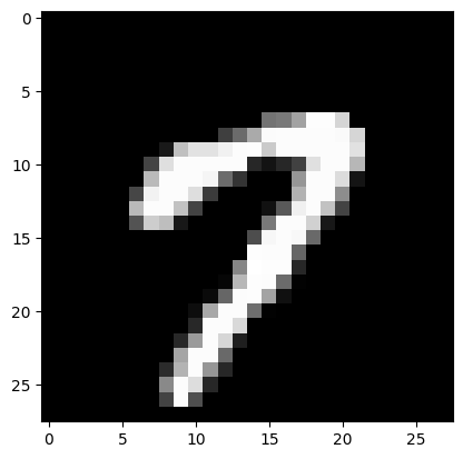
Let us look at a sample image. It is of shape \(28 \times 28\).

img = X[y == 7][0]
img.shape
plt.imshow(img, cmap = 'gray')

<matplotlib.image.AxesImage at 0x7f341659bfd0>

../_images/41cbeafc1342783c0a56dbf15e6bbd45b03ebeb99b6d657387604d9cbc2fd7da.png

This can be treated as a tabular dataset. To do this, we would have to reshape the data-matrix:

print('Original shape', X.shape)
X = X.reshape(60000, -1).T
print('Final shape', X.shape)

Original shape (60000, 28, 28)
Final shape (784, 60000)

We can now treat this as a data-matrix of shape \(d \times n\), where \(d = 784\) and \(n = 60,000\).

NumPy Arrays

Contents

NumPy Arrays#

Arrays#

Reshaping#

Example-1: Vector to matrix#

Example-2: Matrix to vector#

Example-3: Matrix to matrix#

Matrix-vector addition#

Row-vector#

Column-vector#

Advanced Indexing#

Indexing using arrays#

Filtering particular values#

Filtering and follow-up#

Operations along axes#

Top-bottom#

Left-right#

Sum, Mean, Variance, Norm#

Stacking arrays#

Top-bottom#

Left-right#

Misc functions#

Comparing Arrays#

Example#