Ridge Regression#
import numpy as np
import matplotlib.pyplot as plt
Overfitting#
Let us now use the same example that we saw in the previous notebook to study overfitting. In our toy dataset, we shall use \(p = 20\) (where it was \(p = 8\) earlier). Now, we will also have a training and validation dataset. Both of them will have \(n = 20\) data-points, sampled from the same underlying distribution.
Dataset#
rng = np.random.default_rng(seed = 10)
n = 20
x = np.linspace(-1, 1, 2 * n)
p = 20
X = np.array([x ** j for j in range(p + 1)])
y_true = np.sin(2 * np.pi * x)
y = y_true  + rng.normal(0, 0.2, 2 * n)
x_train, X_train, y_train = x[::2], X[:, ::2], y[::2]
x_valid, X_valid, y_valid = x[1::2], X[:, 1::2], y[1::2]
Visualize#
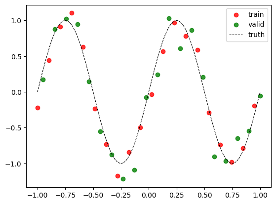
Let us visualize the training data and validation data in the same plot.
plt.scatter(
    x_train, y_train,
    alpha = 0.8,
    color = 'red',
    label = 'train'
    )
plt.scatter(
    x_valid, y_valid,
    alpha = 0.8,
    color = 'green',
    label = 'valid'
    )
x_vis = np.linspace(-1, 1, 200)
y_true_vis = np.sin(2 * np.pi * x_vis)
plt.plot(x_vis, y_true_vis,
         linestyle = '--',
         color = 'black',
         linewidth = 0.8,
         label = 'truth')
plt.legend();
Normal Equations#
We will now use linear regression and see what happens.
w_linear = np.linalg.pinv(X_train.T) @ y_train
Visualize#
Let us now look at the regression curve. We will write this as a function so that we can reuse it later.
def visualize(w):
    plt.scatter(
        x_train, y_train,
        alpha = 0.8,
        color = 'red',
        label = 'train'
        )
    plt.scatter(
        x_valid, y_valid,
        alpha = 0.8,
        color = 'green',
        label = 'valid'
        )
    x_vis = np.linspace(-1, 1, 200)
    y_true_vis = np.sin(2 * np.pi * x_vis)
    y_pred_vis = np.array(
        [w[i] * (x_vis ** i)
        for i in range(w.shape[0])]).sum(axis = 0)
    plt.plot(x_vis, y_pred_vis,
            color = 'red',
            label = 'predicted')
    plt.plot(x_vis, y_true_vis,
            linestyle = '--',
            color = 'black',
            linewidth = 0.8,
            label = 'truth')
    plt.legend()
visualize(w_linear)
plt.ylim(-5, 5);
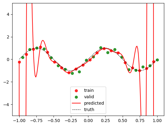
We see the extent of overfitting here visually. We can also study the magnitudes of the weights involved:
print(np.min(w_linear), np.max(w_linear))
-3074832.51598469 2297121.2998212073
We see the huge magnitudes and a wide range. The polynomial is twisting and turning to ensure that it fits the training data as well as it can, in fact, forcing itself to pass through each data-point. But in the process, it ends up fitting the noise as well.
To get a numerical estimate of the extent of overfitting, let us compare the training and test losses.
Loss function#
def loss(X, y, w):
    err = X.T @ w - y
    return (err ** 2).sum() / 2
train_loss = loss(X_train, y_train, w_linear)
valid_loss = loss(X_valid, y_valid, w_linear)
print(f'Train loss = {train_loss}')
print(f'Validation loss = {valid_loss}')
Train loss = 1.2308985803562101e-17
Validation loss = 6193096.573388016
We see that the training loss is zero! The regression curve passes through every data-point!
Ridge regression#
Regualarized Loss function#
Recall that ridge regression tries to minimize the regularized loss function given by:
where \(\lambda\) is the regularization rate.
def loss(X, y, w, lamb):
    err = X.T @ w - y
    return (
        (err ** 2).sum() / 2
        + (lamb / 2) * (w ** 2).sum()
    )
Closed Form Solution#
Since ridge regression makes use of the \(L_2\) loss, we still have a closed form expression for the optimal weight vector:
Since \(\mathbf{XX}^T\) is positive-semidefinite and \(\lambda > 0\), we see that the inverse of the matrix mentioned above always exists.
def get_w_ridge(X, y, lamb = 0.1):
    d, n = X.shape
    return (
        np.linalg.inv(X @ X.T + lamb * np.eye(d))
        @ X @ y
    )
w_ridge = get_w_ridge(
    X_train,
    y_train,
    lamb = 0.01
)
Visualize and Compare#
Let us now visualize the regression curve and also study the training and validation losses.
lamb = 0.01
visualize(w_ridge)
train_loss = loss(X_train, y_train, w_ridge, lamb)
valid_loss = loss(X_valid, y_valid, w_ridge, lamb)
print(f'Train loss = {train_loss}')
print(f'Validation loss = {valid_loss}')
Train loss = 1.5049510776098285
Validation loss = 2.459889499040852
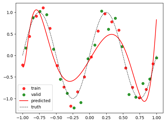
This is a much better model. Note that we are now inching closer to how ML is done in practice. Let us now tune the hyperparameter \(\lambda\) on the validation set. For this, we can plot the training and validation loss against \(\cfrac{1}{\lambda}\).
train_losses = [ ]
valid_losses = [ ]
lambs = np.concatenate([
    [i * (10 ** exp) for i in range(1, 10)]
    for exp in range(-9, 6)]
    )
for lamb in lambs:
    w_ridge = get_w_ridge(
        X_train,
        y_train,
        lamb = lamb
    )
    train_losses.append(loss(
        X_train,
        y_train,
        w_ridge,
        lamb)
    )
    valid_losses.append(loss(
        X_valid,
        y_valid,
        w_ridge,
        lamb)
    )
plt.plot(
    1 / lambs,
    train_losses,
    color = 'red',
    label = 'train'
)
plt.xscale('log')
plt.plot(
    1 / lambs,
    valid_losses,
    color = 'green',
    label = 'valid'
)
plt.xscale('log')
plt.legend()
plt.title(r'Loss vs $1 / \lambda$')
plt.xlabel(r'$1 / \lambda$')
plt.ylabel('Loss')
plt.ylim(0, 10)
(0.0, 10.0)
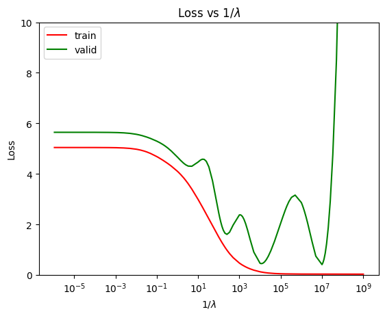
Though this is not a classic curve between the loss function and the model complexity, it at least captures the rough behaviour of the model as \(\lambda\) is varied. In the case of ridge regression, the model complexity is represented by \(1 / \lambda\).
best_lamb = lambs[np.argmin(valid_losses)]
print(f'Best validation loss = {np.min(valid_losses)}')
print(f'Best lambda = {best_lamb}')
Best validation loss = 0.4139661798805553
Best lambda = 1e-07
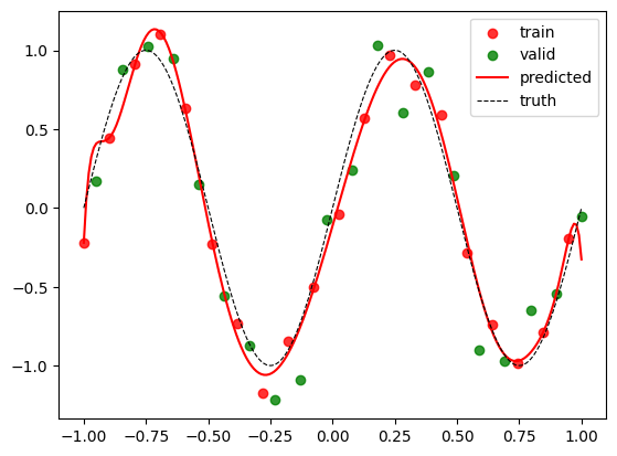
Thus, the best value of \(\lambda\) turns out to be \(10^{-7}\).
w_ridge = get_w_ridge(
    X_train,
    y_train,
    lamb = best_lamb
)
visualize(w_ridge)
train_loss = loss(X_train, y_train, w_ridge, best_lamb)
valid_loss = loss(X_valid, y_valid, w_ridge, best_lamb)
print(f'Train loss = {train_loss}')
print(f'Validation loss = {valid_loss}')
Train loss = 0.03724601299739057
Validation loss = 0.4139661798805553