K-Means Algorithm#
import numpy as np
import matplotlib.pyplot as plt
Toy Dataset#
As before, let us generate a toy dataset.
rng = np.random.default_rng(seed = 138)
mus = np.array([
    [-3, 3],
    [3, -3],
    [3, 3]
])
cov = np.eye(2)
n = 60
xvals = [rng.multivariate_normal(
    mus[i], cov, size = n // 3)
    for i in range(3)]
X = np.concatenate(xvals, axis = 0).T
X = X.astype(np.float32)
X.shape
(2, 60)
Visualize the dataset#
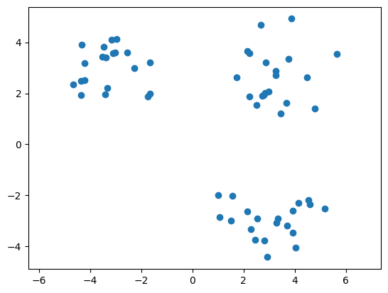
As before, let us visualize the dataset using a scatter plot.
plt.scatter(X[0, :], X[1, :])
plt.axis('equal');
Step-1: Initialization#
Let us choose \(k\) points uniformly at random from the dataset and call them the \(k\) initial means. For this example, we shall use \(k = 3\).
k = 3
d, n = X.shape
ind = rng.choice(
    np.arange(n),
    size = k,
    replace = False
)
mus = X[:, ind]
mus.shape
(2, 3)
mus[:, j] gives the mean of the \(j^{th}\) cluster. The array mus is of shape \(d \times k\). Each column corresponds to a mean.
Step-2: Cluster Assignment#
We will now compute the cluster closest to each point in the dataset and store them in the array \(\mathbf{z}\). Clusters are indexed from \(0\) to \(k - 1\).
z = np.zeros(n)
for i in range(n):
    dist = np.linalg.norm(
        mus - X[:, i].reshape(d, 1),
        axis = 0
    )
    z[i] = np.argmin(dist)
Step-3: Cluster centers#
It is now time to recompute the cluster centers. If a cluster has at least one (actually two) point assigned to it, we need to update its center to the mean of all points assigned to it.italicised text
for j in range(k):
    if np.any(z == j):
        mus[:, j] = X[:, z == j].mean(axis = 1)
K-means function#
We now have all the ingredients to turn this into a function. We need to loop through steps two and three until convergence. Recall that k-means always converges. The convergence criterion is to stop iterating when the cluster assignments do not change. To help with this, we will introduce a new array, z_prev, that keeps track of the previous cluster assignment.
def k_means(X, k = 3):
    d, n = X.shape
    # Step-1: Initialization
    ind = rng.choice(
        np.arange(n),
        size = k,
        replace = False
        )
    mus = X[:, ind]
    z_prev, z = np.zeros(n), np.ones(n)
    while not np.array_equal(z_prev, z):
        z_prev = z.copy()
        # Step-2: Cluster Assignment
        for i in range(n):
            dist = np.linalg.norm(
                mus - X[:, i].reshape(d, 1),
                axis = 0
                )
            z[i] = np.argmin(dist)
        # Step-3: Compute centers
        for j in range(k):
            if np.any(z == j):
                mus[:, j] = X[:, z == j].mean(axis = 1)
    return z.astype(np.int8), mus
Visualize#
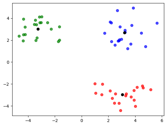
Let us now visualize the clusters we have obtained by running k-means on the toy dataset. The cluster centers are represented in black color.
z, mus = k_means(X)
colors = np.array(['red', 'green', 'blue'])
plt.scatter(
    X[0, :],
    X[1, :],
    c = colors[z],
    alpha = 0.7
    )
plt.scatter(
    mus[0, :],
    mus[1, :],
    color = 'black');
A few additional points related to NumPy. z_prev.copy() does a deep copy in NumPy. To see why we need a deep copy, consider:
a = np.array([1, 2, 3])
b = a
b[0] += 100
print(a, b)
[101 2 3] [101 2 3]
Notice how both a and b change when only b is updated. This is because, both a and b point to the same object. To avoid this, we have:
a = np.array([1, 2, 3])
b = np.copy(a)
b[0] += 100
print(a, b)
[1 2 3] [101 2 3]
The astype method allows us to typecast arrays.
a = np.array([1, 2, 3])
print(a.dtype)
a = a.astype(np.float32)
print(a.dtype)
int64
float32
Image Segmentation#
Let us look at a small application of k-means algorithm: image segmentation. This application is by no means the best way of segmenting images. It is just given here to demonstrate the idea.
import cv2
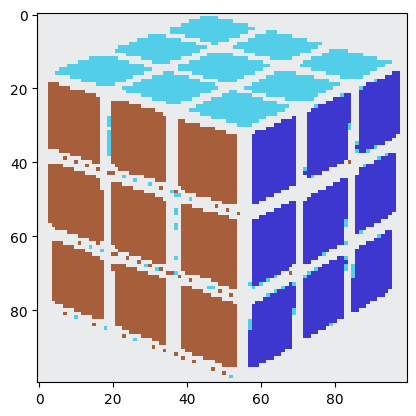
img = cv2.imread('cube.jpg')
plt.imshow(img);
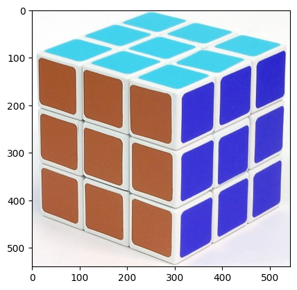
This is rather big. Let us have a more manageable size.
img = cv2.resize(img, (100, 100))
plt.imshow(img);
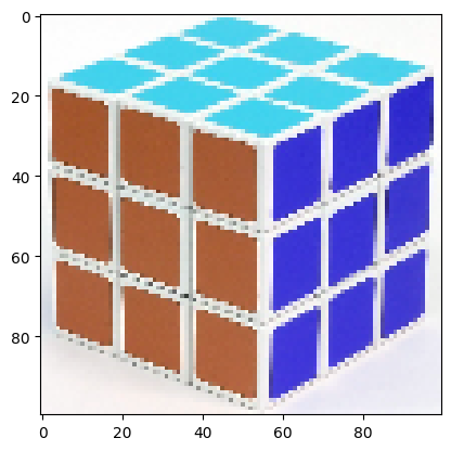
This is a RGB image having \(100 \times 100 = 10,000\) pixels with three channels. We can view this as a dataset of \(10,000\) points in \(\mathbb{R}^{3}\) and run k-means on it. This requires us to carefully reshape the image. For compatibility with some arithmetic operations, let us convert the dataset to float.
img = img.reshape(-1, 3).T
img = img.astype(np.float32)
We now run k-means with \(k = 4\).
d, n = img.shape
rng = np.random.default_rng(seed = 42)
# change seed value to see the effect
z, mus = k_means(
    img,
    k = 4
    )
Let us now replace each pixel in the dataset with the cluster center closest to it.
for i in range(n):
    img[:, i] = mus[:, z[i]]
Let us now reshape the data back into the form of an image and see what we have:
img = img.T.reshape(100, 100, 3).astype(np.uint8)
plt.imshow(img);
It seems as though we have achieved nothing in the process. This image looks, if anything, worse than the original image we had. It is a better idea to run k-means on different kinds of images to see how it segments them.
Image Compression#
But what we have certainly achieved is some kind of compression in storage. Though there are \(10,000\) pixels, we only need to store the following:
\(10,000\) values that represent the cluster indicators for the \(10,000\) pixels
\(4\) means, which is \(4 \times 3 = 12\) values
On the other hand, we had to store \(10,000 \times 3\) values for the original image. This is still a bit vague. So let us take the case of an RGB image with \(n\) pixels, where each pixel is an integer. By running k-means and quantising the image, this is the reduction we get:
we assume that all values are represented as integers. For \(k << n\), this is a compression factor of about \(3\). But clearly, the compression is a lossy compression. Smaller the value of \(k\), greater the information lost.
# Sizes are in bits
int_size = 8 # assuming we use int8
n = 10_000 # num of pixels
k = 4 # num of clusters
num = 3 * n
den = n + 3 * k
np.round(num / den)
3.0
In principle, to store a cluster index, we don’t need an 8-bit int. We can do better by using only \(\log_2(k)\) bits. But for now, we will just stick with int. For a much better example, refer to color quantization using k-means.