Principal Component Analysis#
We will look at a toy dataset first before moving on to a more complex dataset. We will now start using functions wherever applicable so that our code is more modular and reusable.
import numpy as np
import matplotlib.pyplot as plt
rng = np.random.default_rng(seed = 42)
Toy Dataset#
Generate Dataset#
Let us first generate a dataset in \(\mathbb{R}^{2}\) by sampling points from a multi-variate normal distribution.
# Generate Dataset
def generate(mu, cov, n):
    X = rng.multivariate_normal(mu, cov, n).T
    return X

mu = np.array([2, 5])
cov = np.array([
    [1, 0.9],
    [0.9, 1]
])
n = 100
X = generate(mu, cov, n)
X.shape
(2, 100)
Visualise#
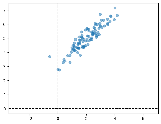
Let us now visualise the dataset using a scatter plot.
def plot(X):
    plt.scatter(X[0, :], X[1, :], alpha = 0.5)
    # alpha controls opacity of the points
    plt.axhline(color = 'black', linestyle = '--')
    plt.axvline(color = 'black', linestyle = '--')
    plt.axis('equal');
plot(X)
Center the dataset#
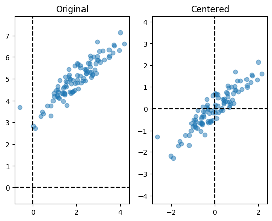
Let us now center the dataset and visualise both the centered and the original dataset side by side.
def center(X):
    mu = X.mean(axis = 1)
    X -= mu.reshape(2, 1)
    return X

plt.subplot(1, 2, 1)
plot(X)
plt.title('Original')
X = center(X)
plt.subplot(1, 2, 2)
plot(X)
plt.title('Centered');
Covariance matrix#
Now, we shall compute the covariance matrix.
def covariance(X):
    d, n = X.shape
    return X @ X.T / n

C = covariance(X)
C
array([[0.87218245, 0.74691674],
       [0.74691674, 0.76626231]])
Principal components#
All that remains is to find the eigenvectors of the covariance matrix, which are our principal components.
def get_PC(C):
    eigval, eigvec = np.linalg.eigh(C)
    eigval = np.flip(eigval)
    eigvec = np.flip(eigvec, axis = 1)
    return eigval, eigvec

var, pcs = get_PC(C)
print('First PC', pcs[:, 0])
print('Variance along first PC', var[0])
print('Second PC', pcs[:, 1])
print('Variance along second PC', var[1])
First PC [-0.7316855  -0.68164237]
Variance along first PC 1.5680143354602323
Second PC [ 0.68164237 -0.7316855 ]
Variance along second PC 0.0704304234954064
# demo of flip
A = np.array([
    [1, 2, 3],
    [4, 5, 6]
])
A = np.flip(A, axis = 1)
A
array([[3, 2, 1],
       [6, 5, 4]])
Visualize PCs#
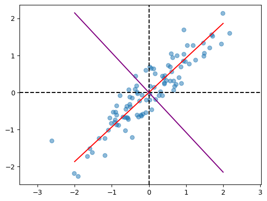
Let us visualize the principal components.
plot(X)
x = np.linspace(-2, 2)
plt.plot(x, pcs[:, 0][1]/pcs[:, 0][0] * x,
        color = 'red',
        label = 'PC-1')
plt.plot(x, pcs[:, 1][1]/pcs[:, 1][0] * x,
        color = 'purple',
        label = 'PC-2');
Summary#
We can now summarize all that we have done and express in the form of two functions.
def PCA(X):
    d, n = X.shape
    # Center
    X -= X.mean(axis = 1).reshape(d, 1)
    # Covariance matrix
    C = X @ X.T / n
    # PCs
    eigval, eigvec = np.linalg.eigh(C)
    eigval = np.flip(eigval)
    eigvec = np.flip(eigvec, axis = 1)
    return eigval, eigvec
def plot(X, pcs):
    # Plot the data
    plt.scatter(X[0, :], X[1, :], alpha = 0.5)
    plt.axhline(color = 'black', linestyle = '--')
    plt.axvline(color = 'black', linestyle = '--')
    # Plot the PCs
    x = np.linspace(-2, 2)
    plt.plot(x, pcs[:, 0][1]/pcs[:, 0][0] * x,
            color = 'red',
            label = 'PC-1')
    plt.plot(x, pcs[:, 1][1]/pcs[:, 1][0] * x,
            color = 'purple',
            label = 'PC-2')
    plt.legend()
    plt.axis('equal');
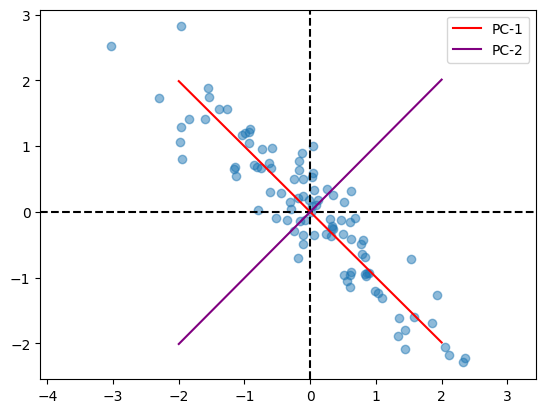
Let us now run PCA for different datasets and see the results.
mu = np.array([2, 5])
cov = np.array([
    [1, -0.9],
    [-0.9, 1]
])
n = 100
X = generate(mu, cov, n)
var, pcs = PCA(X)
plot(X, pcs)
MNIST#
Let us now run PCA on the MNIST dataset and visulize the projections on the top two PCs.
from keras.datasets import mnist
train, test = mnist.load_data()
X_train, y_train = train
print(X_train.shape, y_train.shape)
2024-09-16 22:39:49.883703: I external/local_xla/xla/tsl/cuda/cudart_stub.cc:32] Could not find cuda drivers on your machine, GPU will not be used.
2024-09-16 22:39:49.886720: I external/local_xla/xla/tsl/cuda/cudart_stub.cc:32] Could not find cuda drivers on your machine, GPU will not be used.
2024-09-16 22:39:49.895864: E external/local_xla/xla/stream_executor/cuda/cuda_fft.cc:485] Unable to register cuFFT factory: Attempting to register factory for plugin cuFFT when one has already been registered
2024-09-16 22:39:49.912560: E external/local_xla/xla/stream_executor/cuda/cuda_dnn.cc:8454] Unable to register cuDNN factory: Attempting to register factory for plugin cuDNN when one has already been registered
2024-09-16 22:39:49.917316: E external/local_xla/xla/stream_executor/cuda/cuda_blas.cc:1452] Unable to register cuBLAS factory: Attempting to register factory for plugin cuBLAS when one has already been registered
2024-09-16 22:39:49.930565: I tensorflow/core/platform/cpu_feature_guard.cc:210] This TensorFlow binary is optimized to use available CPU instructions in performance-critical operations.
To enable the following instructions: AVX2 FMA, in other operations, rebuild TensorFlow with the appropriate compiler flags.
2024-09-16 22:39:50.836954: W tensorflow/compiler/tf2tensorrt/utils/py_utils.cc:38] TF-TRT Warning: Could not find TensorRT
(60000, 28, 28) (60000,)
Instead of working with the entire dataset, let us just look at two classes.
y_1, y_2 = 8, 4
print(X_train[y_train == y_1].shape, X_train[y_train == y_2].shape)
(5851, 28, 28) (5842, 28, 28)
Using NumPy’s advanced indexing, we extract the data-points in these two classes.
X = np.concatenate((X_train[y_train == y_1][:100],
                    X_train[y_train == y_2][:100]),
                    axis = 0)
X = X.reshape(X.shape[0], -1).T
X = X.astype(float) # needed while mean subtracting
y = np.concatenate((y_train[y_train == y_1][:100],
                    y_train[y_train == y_2][:100]),
                    axis = 0)
# Change y_1 to 0 and y_2 to 1
y = np.where(y == y_1, 0, 1)
print(X.shape, y.shape)
(784, 200) (200,)
We can now project the data-points onto the top two PCs and visualise the resulting projections in the form of a scatter plot.
var, pcs = PCA(X)
proj = (X.T @ pcs[:, :2]).T
colors = np.array(['red', 'green'])
plt.scatter(proj[0, :], proj[1:, ], c = colors[y]);
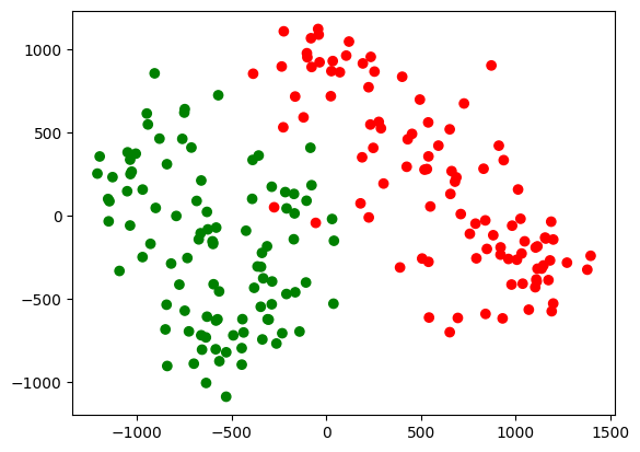
This can now be used in a downstream task such as classification. Notice the neat separation that we get even with just two principal components. This is dimensionality reduction in action.